OpenMusic Tutorials

Prev| Chapter 13. Flow Control III: More Loops!| Next

Tutorial 37: Accumulation with musical objects

Topics

Given a starting note and a melodic sequence, construct a random sequence of notes with the same intervals as the melodic sequence but random directions of motion. Use of a lambda patch within omloop with acum.

Key Modules Used

omloop, Note, Chord-seq, x->dx, om-random, om=, omif

The Concept:

Given a sequence of intervals (B) we will construct a musical sequence starting from a given note (A). The intervals will be ordered as defined but their direction (up or down) will be random (i.e ascending or descending depending on om-random’s output). In order to do so we will use an accumulative proceedure using omloop’s acum collector.

We will also demonstrate the sequence function by simultaneously visualizing our new melodic figure using a BPF factory.

The Patch:

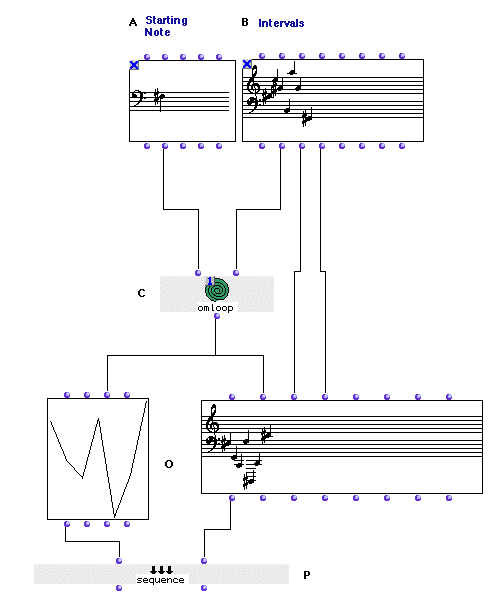
The transformation of the sequence into a new one will be done in omloop (C). This transformation is a transformation of pitch only, so omloop (C) is connected to the second input of Chord-seq (O). To get the rhythmic data we take the _ldur_ and _lonset_ outputs of the Chord-seq (B) and copy them directly.

omloop as shown above is in ‘eval-once’ mode. This is because omloop is connected to two objects but contains a random function. We want to make sure the same information is given to both the Chord-seq and the BPF, which will not happen unless we ‘freeze’ it after one evaluation.

Now let’s look inside omloop.

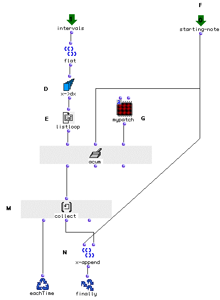
First of all we must convert the list of midics we will be receiving through the _intervals_ input into a list of relative intervals. This is done, as usual, using x->dx. We must first use flat since the _lmidic_ output of the Chord-seq is a nested listand x->dx needs a flat list.

Each interval of the Chord-seq will thus be enumerated individually and passed to our lambda patch (G) along with the results of the previous calculation.

Here’s the lambda patch:

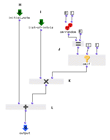
The lambda patch (G) will take the initial note (H) and will add to it the first interval (I). This interval will have been first multiplied either by 1 (which will leave it as is) or by -1 (which will invert the interval.)

In order to randomly invert the intervals we have used om-random. As we know, om-random returns random numbers between limits set at its inputs. In our case we had to use a different strategy because we are only interested in having -1 and 1. Simply using om- random could have returned some zeroes. This is where omif comes in handy. We used om-random with 0 and 1 as arguments and connected it to the predicate om=in order to transform each zero into a -1. If om-random returns a zero, om= will return t and omif, in turn, will return -1. If not, 1 is returned.

Once we have added our first interval (using om+) to the initial note, the result will be a new note which will take the place of the old as the internal state of our acum collector. In order to record each note we use collect, connected to the first output of acum, as we did in the previous tutorial.

Lastly, in order to have both factories (the BPF and the Chord-seq) evaluated in a single evaluation we will use sequence. sequence evaluates all its arguments sequentially, but you will only see one in the Listener. For instance, if we evaluate the first output of sequence we will obtain the BPF object in the listener. Evaluating the second output will return the Chord-seq object. Both will be evaluated in the patch window, however.

OpenMusic